A tutorial for using CLUZ with QGIS

Exercise 2: Producing the CLUZ files

CLUZ is a plugin for QGIS that lets people design conservation landscapes and seascapes based on the principles of systematic conservation planning. It can be used for on-screen terrestrial and marine spatial planning and also acts as a link for the Marxan and Marxan with Zones spatial prioritisation software packages. CLUZ was funded by the UK Government’s Darwin Initiative.

This exercise shows how to produce the CLUZ files that you used in Exercise 1. The first part shows how to create these files and the second and third parts show how to update these files based on the available abundance and conservation status data.

It is worth noting that when creating new files, QGIS is very stringent when it comes to the quality of input files and will not ignore errors with vector geometry. This is in contrast to other GIS software packages that ignore the errors, producing error-filled results without flagging up the problems. When using your own vector files, you can check for problems using the Vector> Geometry Tools> Check Validity modules and fix any errors using a range of tools provided by QGIS.

Part 2a: Creating the planning unit shapefile, target and abundance data

In this section you will produce the blank files that CLUZ needs to operate.

1) Get the tutorial files from https://anotherbobsmith.github.io/cluz.html by downloading the cluz_ex2.zip file (your Internet browser may warn you about downloading zip files but these CLUZ files are safe). Unzip the files and save the cluz_ex2 folder on your computer in a suitable location.

CLUZ Exercise 2 data (cluz_ex2.zip)

2) Click on the Open Data Source Manager and choose to add a Vector layer . Add the nature reserve and hexagons shapefiles (.shp) from the cluz_ex2 folder to the View and display them. You will see the nature reserve layer shows the boundary of a protected area and the hexagons layer shows a number of 25 ha hexagons that have been clipped the planning region boundary. Hexagonal planning units are often used in conservation planning exercises but planning units can be any shape. Remove the two shapefiles from the View.

Now add the planning units layer from the \cluz_ex2 folder to the View. This was produced by using the Union function in QGIS to combine the nature reserve and hexagons layers and then deleting some tiny slither polygons that were created during the union process. Notice how each planning unit is a hexagon or a section of a hexagon if it crosses the nature reserve or planning region boundary. Make the planning units layer active and click on Open Attribute Table button and notice that the table only contains fields called Name and Region. Close the table and remove the planning units layer from the View.

3) Next you will create the CLUZ files by modifying the planning unit layer and creating the puvspr2.dat and target files. In the CLUZ menu choose Create initial CLUZ files. Click on the Select shapefile Browse button and select the planning units layer. Set the Area conversion factor as 10000 as this will convert the Area values from m² to hectares. Click on the Set cost layer as equal to planning unit area. Set the input folder where the puvspr2.dat file will be stored as \cluz_ex2\input and specify that the target table should be named targets.csv and saved in the \cluz_ex2 folder. Click on OK.

Once the process has finished, add the planning units layer to the view again. Click on the Open Attribute Table button again. Notice that CLUZ has added fields named Unit_ID, Area, Cost and Status. You will see that the unique Unit_ID value is set as the row number and that the Cost value is the same as the Area value (which will be 25 ha for the whole hexagons). Close the table and remove the planning units layer from the View.

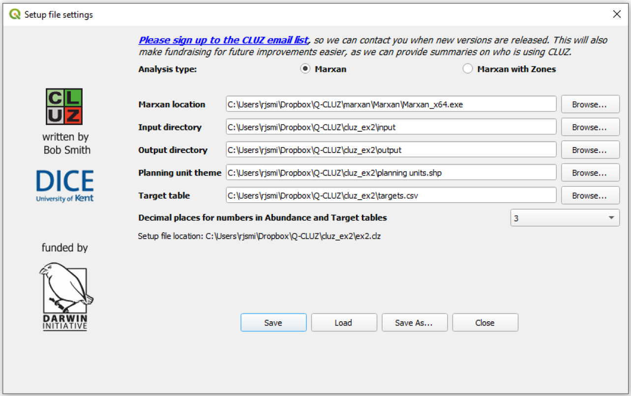
4) You have now created the files that CLUZ needs to undertake conservation planning. The puvspr2.dat and targets.csv files are blank but contain the required fields. In the later steps you will modify these tables but you must first create a CLUZ setup file. Do this by choosing View and edit CLUZ setup file from the CLUZ menu.

Repeat the process you learnt about in Exercise 1. Click on the Browse buttons to set the different input parameters. These should be identical to those shown in the figure associated with Exercise 1b part 3, except the specified folder for the CLUZ files should be \cluz_ex2 not \cluz_ex1. Use the Save As button to save the setup files as ex2.clz in the cluz_ex2 folder.

Now click on the Open Target Table button and note that the table does not contain any data yet. Close the table to return to the View.

Part 2b: Updating the status of the planning units

In this section you will update the Status information in the planning units layer. In particular, you will specify that planning units near to two proposed economic “growth points” should be Excluded and planning units within the nature reserve should be set as Conserved.

1) From the \cluz_ex2 folder add the layer called growth_points.shp to the View. You will exclude all planning units that are within 2 km of these points, so the first step is to produce a layer showing the area that falls within this distance. In the QGIS menu Vector > Geoprocessing Tools choose Buffer… . Set the Input layer as the growth points layer, the Distance as 2000, the Segments as 50 and leave the other parameters as the default. Click on Run and then Close. You should see that a layer named Buffered has been added to the View.

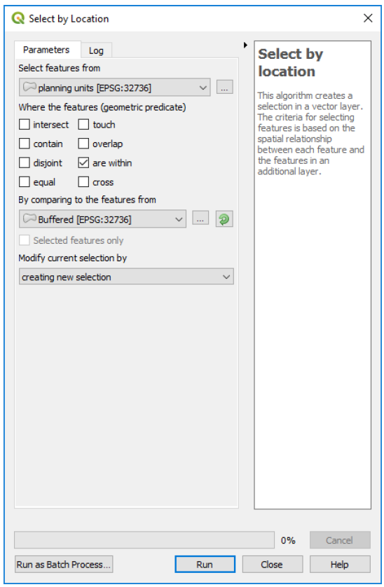
Now got to Vector > Research Tools > Select by Location. For the Select features from section choose Planning units. For the section on Where the features (geometric predicate) click on the tickbox for are within. For the By comparing to the features from choose Buffered. Now click on Run and then Close. In the View, turn off the Buffered layer and underneath you should see that 73 planning units have been selected and are shown in yellow.

2) Now click on the open the Change Status Panel button and click on the Allow changes to Conserved and Excluded status tick box . This will display the Conserved and Excluded radio buttons, so select the Excluded radio button and click on the Change button.

The selected units will now be coloured in purple to show they have Excluded status and will not be included in any portfolio selected by Marxan. Close the Change Status panel and remove the growth_points and Buffered layers from the View.

3) The next step is to set the status of the Conserved units and this involves identifying the planning units that fall within the nature reserve. Make the planning unit layer active and click on the Open Attribute Table button . Once the table is open, click on the Select features using an expression button . In the Expression box type "NAME" = 'Ithemba' and click on the Select features button at the bottom of the dialog box. This will have selected all the planning units that belong to the nature reserve, which is called Ithemba and named in the original nature reserve layer. Close the dialog box, then close the attribute table and return to the View. You should see that all the planning units within the protected area have been selected and are shown in yellow.

Now click on the Open Change Status Panel button again and click on the Allow Changes to Conserved and Excluded status tick box . This time select the Conserved radio button and click on the Change button.

Part 2c: Adding abundance data and updating the target table

You can use CLUZ to import data on the distribution of your conservation features, either by extracting the data from raster layers and shapefiles or using data that has been produced through other methods. In this section, you will extract landcover data from a raster file, plant distribution data from a vector file and will import bird distribution data from a csv file.

1) Click on the Open Data Source Manager and choose to add a Raster layer . Add the raster layer landcover.gpkg from the \cluz_ex2 folder. This layer shows the distribution of 18 landcover types, so each pixel has a value corresponding to the unique ID value of these 18 conservation features (the ID values range from 1 for Montane aquatic to 33 for Open Water). By default, QGIS shows this layer with a greyscale palette so if you want to change this, open the layer’s Properties dialog box and in the Symbology tab change the Render type to Palleted/Unique values and then click on the Classify and OK buttons.

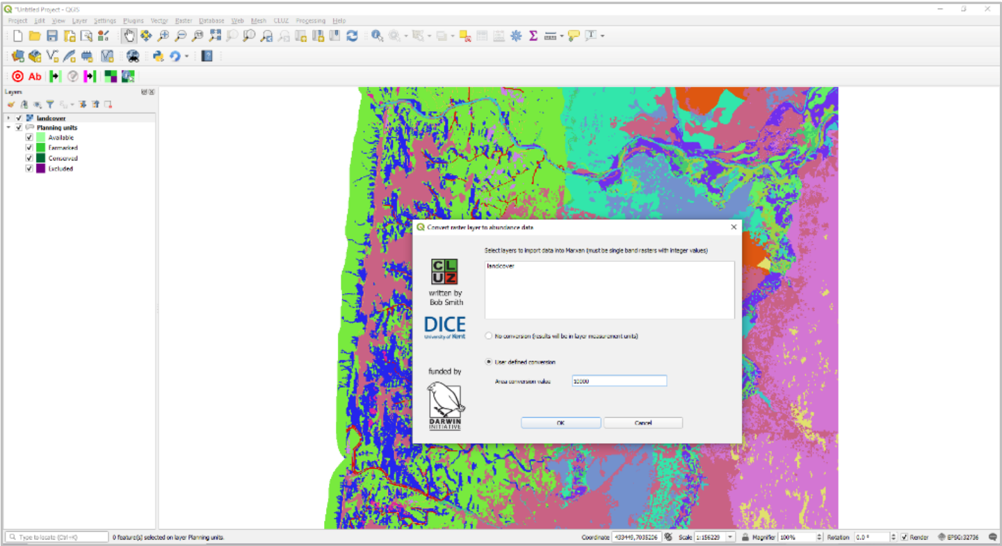
From the CLUZ menu, select Convert raster layer to Marxan abundance data. This calculates the amount of each feature in each planning unit and then imports the data into the targets.csv and puvspr2.dat files. Select landcover as the layer to import, turn on the button and set the value as 10000 to convert from m² to hectares. Click OK.

Check the data have been imported correctly by clicking on the Open abundance table button and selecting all the features. Close the abundance table. Open the target table and notice that 18 new rows have been added to the table and the numerical identifier of the added features has been added to the Id field. CLUZ has also calculated the total amount of each feature found in the planning region, and the total amount in Earmarked and Conserved planning units. The Name, Type, Target and Spf values are blank but you will fill those in later. Close the table and remove the landcover layer from the View.

2) CLUZ can also be used to extract distribution data from shapefiles and to demonstrate this add the theme called cycads.shp from the \cluz_ex2 folder. The cycad theme shows the distribution of two plant species, one of which is found in two areas in the northwest and southwest.

Make the theme active and click on the Open Attribute Table button and notice that the table contains a field called ID containing the ID values 105 and 107. All themes you wish to incorporate must contain a numeric field that contains the unique identifiers for each conservation feature.

Close the table and in the CLUZ menu choose the Convert polyline or polygon themes to Marxan abundance data module. Select cycads.shp as the theme you want to use, leave the default value that the Layer ID field name is ID, turn on the button and set the value as 10000 to convert values from m² to hectares.

3) Now you will add data on the presence of vulture nests using the Import fields from table to Marxan abundance file option. The file nest_data.csv contains a count of the number of nests per planning unit so use the Browse button to specify the file and set the Layer ID field name as Unit_ID. Choose the because this is count data and does not need to be converted. Then click on OK

4) Click on the Open target table button and you will see the new features have been added and the cycad species have ID values of 105 and 107, whilst the vulture nest ID value is 156. You now need to add the relevant data on each of the 21 conservation features and you will do this in Excel. Open the targets.csv file that you created and the feature_details.csv file that are in the /cluz_ex2 folder.

Copy the conservation feature names, types, SPF values and targets from the feature_details.csv file, based on their ID values. The type codes are based on whether the feature is a man-made landcover type (Type 0), common natural landcover type (Type 1), an endemic or threatened landcover type (Type 2) or a species (Type 3). The SPF values are used by Marxan and must be set as higher than 0 (see the Marxan manual for more details). The targets reflect the conservation value of each feature.

Save the data in your targets.csv file by clicking on the Save button and selecting Yes. Close the file in Excel and in CLUZ click on the Open target table button . You should now see the updated information that you added and the PC_target field automatically updates to show how well the targets have been met.