A tutorial for using CLUZ with QGIS

Exercise 3: Using CLUZ to run Marxan with Zones

CLUZ is a QGIS plugin that lets people design conservation landscapes and seascapes based on the principles of systematic conservation planning. It can be used for on-screen terrestrial and marine spatial planning and also acts as a link for the Marxan and Marxan with Zones spatial prioritisation software packages. CLUZ was funded by the UK Government’s Darwin Initiative.

Exercise 1 of these tutorials showed how to run Marxan through CLUZ and Exercise 2 showed how to create the files needed to run Marxan. Marxan is designed to identify which new areas should be added to a conservation area network. This involves dividing up the planning region into a series of planning units and selecting the best set planning units for meeting conservation targets, whilst minimising costs and maintaining connectivity. In effect, this means Marxan assigns each planning unit to one of two management zones: a conservation zone and a business-as-usual zone.

In the real world, we often want to develop ecological networks consisting of more than two zones. For example, we might want to distinguish between different types of conservation zone or include zones for habitat creation and restoration. Marxan with Zones was developed for exactly this type of situation and can also be run through CLUZ. This exercise shows how to produce the Marxan with Zones files and then run a simple Marxan with Zones analysis. If you are not familiar with using CLUZ to run Marxan, we strongly recommend that you complete Exercise 1 and Exercise 2 first.

Part 3a: Converting the CLUZ files into Marxan with Zones format

The process for producing Marxan with Zones files is based on setting everything up in the Marxan format and then transforming it into the Marxan with Zones format. In this section you will produce the files that CLUZ needs by transforming the files used in Exercise 1 into the Marxan with Zones format.

1) This exercise uses the tutorial files that are produced as part of Exercise 1. To set up these files, you need to at the very least complete sections 1a and 1b of Exercise 1 (although we recommend completing the whole exercise). If you follow the instructions in Exercise 1 fully then you should produce a file named ex1.clz and saved it in the \cluz_ex1 folder. This file lists the locations of all the files used by CLUZ and Marxan.

2) Before you open QGIS, create a folder named cluz_ex3 in the same directory as the cluz_ex1 folder. This is where you will save the Marxan with Zones input and output files. You also need to download and unzip Marxan with Zones HERE.

3) Open QGIS and make sure the CLUZ plugin is installed. In the CLUZ menu choose View and edit CLUZ setup file and click on the Load button. Select the ex1.clz file that you produced in Exercise 1 and CLUZ will display the five pathways of the different files and folders. Click on the Close button and you will see that CLUZ has automatically added the planning unit shapefile to the QGIS Table of Contents.

4) You are now ready to convert these files from Marxan to Marxan with Zones format. In the CLUZ menu choose Transform CLUZ files from Marxan to Marxan with Zones format. Start by clicking on the Browse button next to the Marxan with Zones location input. Navigate to the folder where you saved Marxan with Zones and, if you are using Windows computer, choose MarZone_x64.exe (for other operating systems you will have different options).

Next click on the Browse button next to Empty folder for new files and specify the location of the cluz_ex3 folder you created in Step 2 above.

Change the name of the New Marxan with Zones setup file name from zones_ex1 to ex3 but keep the default names for the planning unit layer, the target file and the zone file. Also keep the number of zones to be created as the default number of 3. Click on OK.

CLUZ has now produced the Marxan with Zones files, so close QGIS.

Part 3b: Updating the target and zones table files

This tutorial is based on designing an ecological network based on three zones. Zone 1 will be for protected areas, which will be managed for biodiversity and receive the highest levels of conservation funding and protection. Zone 2 will be for OECMs (other effective area-based conservation measures), which will be managed for community-based ecotourism and have lower levels of anti-poaching activity. Zone 3 will be for the rest of the landscape and will have no specific conservation management.

5) Using Windows Explorer, look at the files created in the cluz_ex3 folder. You will see the input folder, which contains the puvspr2.dat file copied over from Exercise 1 that lists the amount of each feature in each planning unit. You will see the output folder, which is currently empty. You will see the files that make up the planning unit shapefile (named zones_puLayer), the target files (named zones_targets.csv) and the zones file (named zones_details.csv). You will also see the ex3.clz file that specifies the locations of these other files and is used by CLUZ.

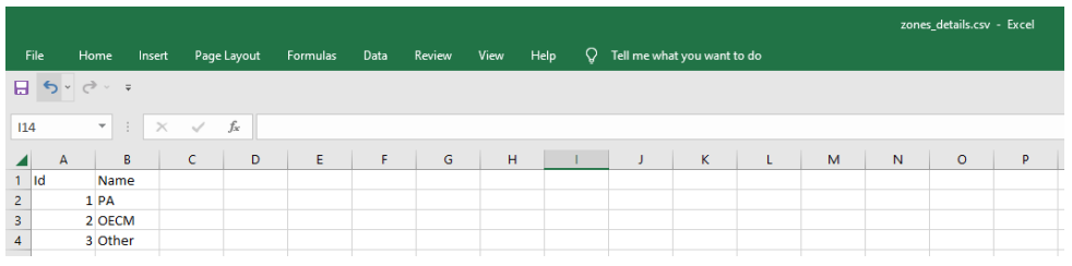
6) The zones file is a simple csv file that lists the numerical id value of each zone and their names. As a first step, open this zones_details.csv file and change the name of each zone from Blank to PA for Zone 1, OECM for Zone 2, and Other for Zone 3. Save your changes.

7) Open QGIS and in the CLUZ menu choose View and edit CLUZ setup file. Load the ex3.clz file and notice the paths names of the different files that you created above. Close the dialog box.

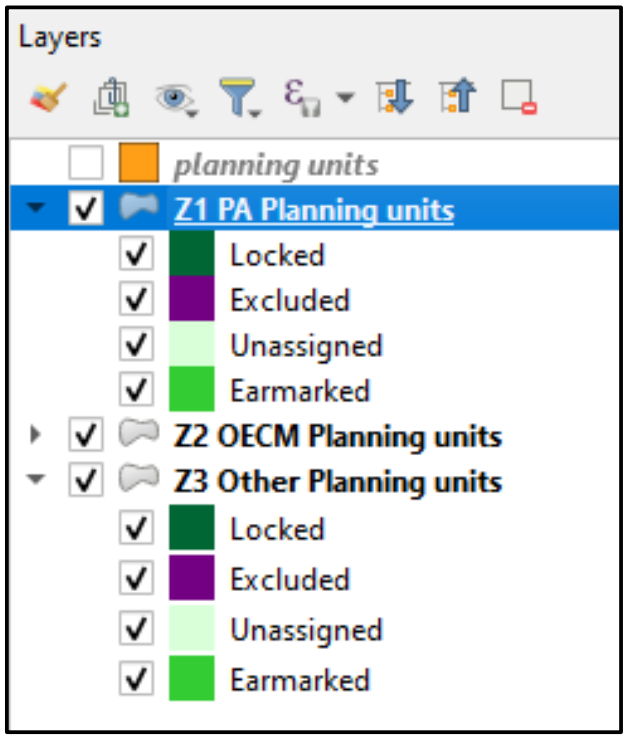
The CLUZ file system is based on only having one planning unit theme and this is still the case when using Marxan with Zones. So, you will see that CLUZ has added three copies of the planning unit layer, one for each zone and named Z1 PA Planning units, Z2 OECM Planning units and Z3 Other Planning units.

You will also see the legends for each layer show that for Marxan with Zones, CLUZ uses slightly different names for the status of each planning unit: Locked, Excluded, Unassigned and Earmarked. At the moment, every planning unit in all three zones has Unassigned status.

8) Another addition to CLUZ for Marxan with Zones is that the Open Zones Table button is active. Click on this button to see a table showing the id values and names that you specified in the zones_details.csv file. Close the table.

9) Click on the Open Zones Table button. You will see the same list of features from Exercise 1 but a number of new fields have been added, all given default values at this early stage. The Z1_Prop, Z2_Prop and Z3_Prop fields specify the proportion of that feature that counts towards targets if a planning unit is assigned to the associated zone. This will be explained in more detail below.

The Z1_Target, Z2_Target and Z3_Target fields specify zone specific targets, which will also be explained in more detail below. The Z1_Ear+Lock, Z2_Ear+Lock and Z3_Ear+Lock fields show the contributing amount of each feature in planning units with Earmarked or Locked status in each zone. At present, all these values are 0 because every planning unit has Unassigned status.

Close the Target table.

Part 3b: Updating the planning unit files

This tutorial is based on designing an ecological network based on three zones. Zone 1 will be for protected areas, which will be managed for biodiversity and give the highest levels of protection. Zone 2 will be for OECMs (other effective area-based conservation measures), which will be managed for community-based ecotourism and have lower levels of anti-poaching activity. Zone 3 will be for the rest of the landscape and will have no specific conservation management

1) Right click on the Z1 PA Planning units layer in the Table of Contents and select the Open Attribute Table option. You will see that the table has eight fields. The Unit_ID field gives the unique identifier for each planning unit and the Area field the area of each planning unit. The other fields describe the cost and status of each planning unit in each zone. At present, all the cost values are 0 and all the status values are Unassigned. Close the Attribute table.

2) You will now update the planning unit status details, copying information from the Exercise 1 layer. In Exercise 1, some planning units were in a nature reserve and set as conserved (always selected in Marxan) and some were going to be converted to housing and set as excluded (never selected by Marxan). You will treat them differently in this exercise, illustrating one of the main differences between using Marxan and Marxan with Zones. In this exercise, you will lock-in the nature reserve planning units into Zone 1 and lock-in the proposed housing planning units into Zone 3.

Click on the Open Data Source Manager and choose to add a Vector layer. Add the planning unit shapefile (planning_units.shp) from Exercise 1. Next double-click on the Z1 PA Planning units layer in the Table of Contents to bring up the Layer Properties dialog box. Select Joins and click on the Add new join button. For the Join layer, select planning units, for the Join field select Unit_ID and for the Target field select Unit_ID. Click on OK to make the join and click on OK again to close the Layer Properties dialog box.

3) Right click on the Z1 PA Planning units layer in the Table of Contents and select the Open Attribute Table option again. You will see that the fields from the Exercise 1 planning units have been temporarily added, (planning units_Area, planning units_Cost, etc). You will use this information to update the planning unit status values in each zone.

Close the attribute table.

4) First you will update the status of planning units in Zone 1. Make the Exercise 1 planning units layer invisible by clicking off its checkbox in the Table of Contents. Make the Z1 PA Planning units layer active by clicking on it in the Table of Contents so it has a blue bar around it (as shown in the figure to the right). QGIS will now update the information in this selected shapefile (although the Z1, Z2 and Z3 planning units are copies of the same file, so any changes you make to the attribute tables will be applied to all of them).

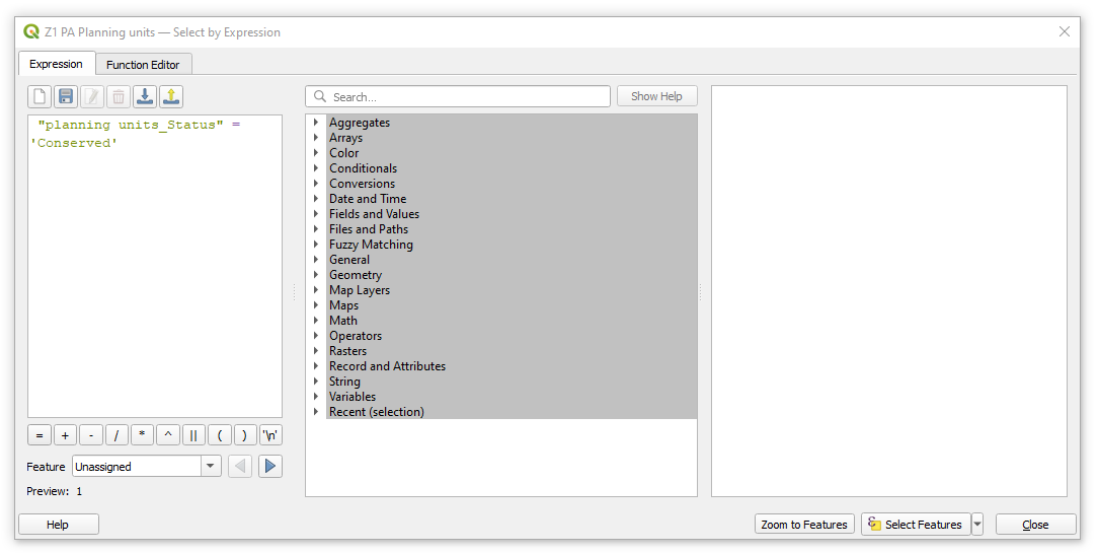
In the main menu bar, click on the Select Feature by Expression button. In the Select by Expression dialog box, type "planning units_Status" = 'Conserved' into the Expression box and then click on the Select Features button. Make sure the text is exactly the same as that shown below in the screen shot from the Select by Expression dialog box. Close the dialog box to see how it has updated the layer.

5) The Z1 PA planning units in the north-east of the planning region will now be shown in yellow. Click on the Change Status panel and make sure the Zone name is Zone 1 – PA. Click on the Allow changes to Locked and Excluded status tick box and then specify Set as Locked In. Click on the Change button and you will see that the selected planning units are shown in dark green, indicating that they have Locked in status. Click on the Close button.

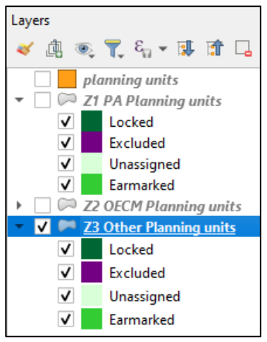
6) Next you will update the status of planning units in Zone 3. Make the Z1 PA planning units and Z2 OECM planning units invisible by click off their tick boxes in the Table of Contents, so you can see Z3 Other planning units below. Make the Z3 Other Planning units layer active by clicking on it in the Table of Contents so it has a blue bar around it (as shown in the figure to the right).

You will now join the Exercise 1 planning unit details to this Z3 planning unit layer. Double-click on the Z3 Other Planning units layer in the Table of Contents to bring up the Layer Properties dialog box. Once again, select Joins and click on the Add new join button. Again, for the Join layer, select planning units, for the Join field select Unit_ID and for the Target field select Unit_ID. Click OK to make the join and click OK again to close the dialog box.

7) Once again, click on the Select Feature by Expression button but thin time type "planning units_Status" = 'Excluded' and then click on the Select Features button.

8) There will be two patches of selected Z3 Other planning units in the centre of the planning region shown in yellow. Click on the Change Status panel and make sure the Zone name is Zone 3 - Other. Click on the Allow changes to Locked and Excluded status tick box Click on the Change button and you will see that the selected planning units are shown in dark green. Click on the Close button.

You have now updated the status values in the three zones so that they replicate the situation in Exercise 1.

9) You will nest update the cost values in each of the Zone cost fields, starting with Zone 1. In the Table of Contents, right click on the Z1 PA planning units layer and choose Open Attribute Table. Click on the Toggle editing mode button and then the Open Field Calculator button. Click on the Update existing field tick box and from the drop-down menu underneath choose Z1_cost. In the Expression box type Area to make the Zone 1 cost the same as the values in the Area field (i.e., the planning unit area measured in hectares). Click on OK.

10) Now repeat the process to add the values for Zone 2, but this time you will reduce the costs by 50% to reflect that it is cheaper to manage OECMs (this is a relatively crude way of representing these lower costs. In real-world conservation planning you will probably want to use something more sophisticated). Click on the Open Field Calculator button again, click on the Update existing field tick box and from the drop-down menu underneath choose Z2_cost. In the Expression box type "Area" / 2 to make the Zone 2 costs half the values in the Area field. Click on OK.

11) The planning unit cost values represent the cost of adding land to the ecological network. This means that the Zone 3 cost values should be different, as they will not be managed for conservation or restoration. Thus, the cost of each planning unit when assigned to Zone 3 is basically zero, but it is good practice to give every planning unit a cost greater than 0 to reflect that adding to a zone is never completely cost free. So, click on the Open Field Calculator button, click on Update existing field and choose Z3_Cost, but this time specify in the Expression box that the value should be 0.001. Click on OK.

You have now finished editing the attribute table, so click on the Save edits button and the Toggle editing mode button. As a final check, make sure that for the planning unit with a Unit_ID value of 1 the cost values are 7.040 for Zone 1, 3.520 for Zone 2 and 0.001 for Zone 3. Close the attribute table and return to the QGIS View.

Part 3c: Updating the proportion values and targets

1) Click on the Open Zones Table button. You will see that the values have been updated to show how much of each feature is in Ear+Lock (Earmarked or Locked) planning units in each zone, based on changing the status of planning units in Zone 1 and Zone 3. However, Zone 3 will not be managed for conservation and so should not contribute to the targets. Similarly, in this exercise we want to distinguish between the contribution of Zone 1 and Zone 2 to represent the fact that in our example, OECMs will only contribute to landcover type targets.

CLUZ and Marxan with Zones lets the user specify the extent to which different zones contribute towards each feature’s target through their proportion values. These values are specified in the Prop fields. For a hypothetical example based on giraffes, if a planning unit contains potential habitat for 20 giraffes, we could specify a Z1_Prop value of 1.0 to indicate that 20 giraffes will be found in the planning unit if it is assigned to the PA zone, a Z2_Prop value of 0.5 to indicate that 10 giraffes will be found in the planning unit if it is assigned to the OECM zone and a Z3_Prop value of 0.0 to indicate that 0 giraffes will be found in the planning unit if it is assigned to the Other zone.

2) For this exercise, we will assume that if a planning unit is assigned to the PA zone, then all the important conservation features will be fully conserved, so their total amount will count towards the targets. But for the OECM zone only the important landcover features will be fully represented; the species features will be absent because they need high levels of anti-poaching management. The Other zone will not contribute to any of the feature targets.

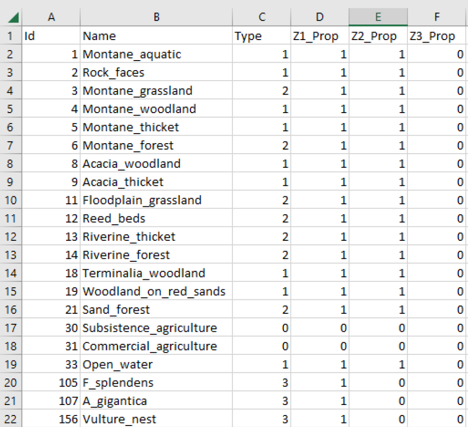
To edit the target table, open the zones_targets.csv file in Excel or a similar software package. Edit the Prop fields, based on the information in the Type field. The Type field has four values: 0 for landcover types with no conservation value, 1 for landcover types with medium conservation value, 2 for landcover types with high conservation value and 3 for species with high conservation value.

In the Z1_Prop field, for Type 0 change the value to 0, i.e., for Subsistence agriculture and Commercial agriculture set a value of 0.

In the Z2_Prop field, for Type 0 and Type 3 change the value to 0, i.e., for Subsistence agriculture, Commercial agriculture, F splendens, A gigantica and vulture nests set a value of 0.

In the Z3_Prop field, set all the values to 0. The final table should look like the figure above.

3) In this exercise, you will keep the values in the Z1_Target, Z2_Target and Z3_Target fields as 0. This is because we are only interested in the combined amount conserved in Zone 1 and Zone 2 and so do not need to set targets for specific zones.

You can now save the changes to the zones_targets.csv file and close it.

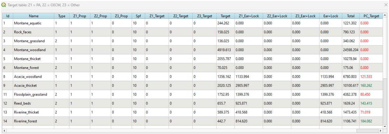
4) Return to QGIS and click on the Open Zones Table button to check the changes. The first rows of the target table should look like the figure below.

Notice that the amount of each feature in the Z3_Ear+Lock field is now 0. This is because you set every Z3_Prop value to 0, and the Ear+Lock value equals the potential amount of the feature found in the Earmarked and Locked planning units multiplied by the proportion value for that zone.

This is also reflected in the Ear+Lock field, which sums the values in the Z1_Ear+Lock, Z2_Ear+Lock and Z3_Ear+Lock fields. The PC_Target field shows the values in the Ear+Lock field divided by the values in the Target field, so also accounts for the proportion values given to each feature for each zone. If the PC_Target value is 100% or more then this means the target has been met and the value is shown in green.

Part 3d: Running Marxan with Zones

In the previous sections you converted the CLUZ files from Marxan to Marxan with Zones format, updating the planning unit status values and adding data for each of the three zones on the planning unit costs and the proportion of each feature that counts towards the targets. In this section you will learn how to create the Marxan with Zones files and use them to run several different analyses.

1) In the CLUZ menu, choose Create Marxan input files. Because you are doing this for the first time, click on all four checkboxes to produce the Target and feature files, Planning unit files, Zones files and Boundary file. DO NOT click the Include planning region boundaries checkbox, so that the edges of units that are not shared (i.e., form the boundary of the study region) are not included in the boundary.dat file. Including the external edges makes it less likely Marxan with Zones will select planning units at the edge of the planning region.

Click on the OK button. The Create Marxan input files function will use the data from the CLUZ planning unit layer, target table and zones table, so if you change these data in the future you will need to update the corresponding Marxan files by running it again.

2) Using Windows Explorer, look at the files created in the input folder within the cluz_ex3 folder. There should be 12 text files, all with the .dat suffix. This is considerably more than the four files needed to run Marxan. This illustrates the added complexity that Marxan with Zones was designed to incorporate into the spatial prioritisation process.

3) Return to QGIS and in the CLUZ menu, choose Launch Marxan. In this tutorial you will use these default values to reduce the time Marxan spends processing the data. Use output1 as the Output file name and leave the Include boundary cost (BLM) and Produce extra Marxan outputs checkboxes unchecked . The Produce extra Marxan outputs option saves files describing the results from each run, which are not needed for this exercise.

Click on Start Marxan with Zones and the Marxan with Zones dialog box should appear. The dialog box will show the data are being inputted and will give details on each of the 10 runs.

NB If you are running CLUZ on a computer with high security settings, your system might not let CLUZ run Marxan with Zones. If that happens Marxan with Zones will produce the error message “Input file input.dat not found. Aborting program” and/or it will look as though it has frozen. To overcome this problem, you can run Marxan with Zones yourself by using Windows Explorer to locate the Marxan with Zones file (the file path is specified in your CLUZ setup file) and double clicking on it. Marxan with Zones should now run and, once finished, CLUZ will display the results.

4) Once Marxan with Zones has run, CLUZ will add four output layers to the QGIS View. The Best (output1) layer shows the best Marxan with Zones output, i.e., the output with the lowest cost from the 10 runs. The best output assigns each planning unit to one of the three zones, so you will see: the existing protected area is assigned to Zone 1, together with a scattering of planning units that include the ranges of the three species; planning units assigned to Zone 2 are scattered across the planning region, and; most planning units are assigned to Zone 3, including those that were locked-in because they are unsuitable for conservation (Figure 1).

The other three output layers show the selection frequency scores for each of the three zones. The planning units selected in each of the ten runs are shown in red, so include the locked-in planning units for each zone (Figure 1).

Right click on the Z1 PA Planning units layer in the Table of Contents and select the Open Attribute Table option again. You will see that CLUZ has added four fields to the attribute table containing the data displayed in the four outputs – Best, Z1_SFreq, Z2_SFreq and Z3_SFreq. The data in these fields is replaced every time you run Marxan with Zones to reflect the latest results.

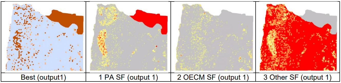Figure 1: An example of the four output layers produced by CLUZ to display the Marxan with Zones outputs, based on ten runs, 1,000,000 iterations and with a Boundary Length Modifier value of 0. Marxan with Zones will produce different results each time it is run, but for this analysis your results should be similar.

5) The previous results produced very fragmented results, so from the CLUZ menu choose Launch Marxan again. Use all the default options once again, except this time click on the Include boundary cost (BLM) checkbox and set the BLM value as 0.2. Click on Start Marxan with Zones and the Marxan with Zones dialog box will appear. Once again, CLUZ will display the best and the selection frequency outputs for the three different zones. You will see that the patch sizes of each zone are now much larger (Figure 2 gives examples, your results will be different but similar).

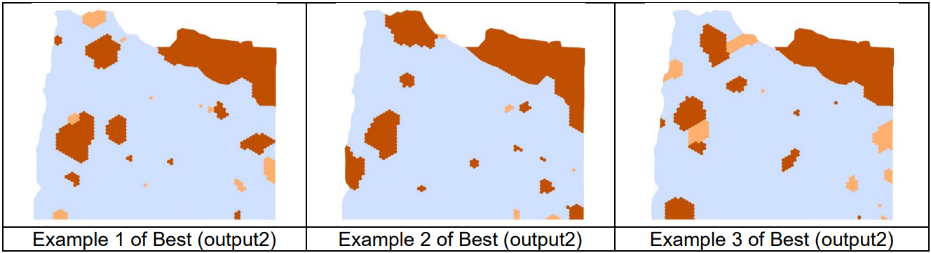Figure 2: Three different examples of the Best (output2) layer produced by CLUZ, based on ten runs, 1,000,000 iterations and with a BLM value of 0.2. Marxan with Zones produces different results each time it is run, so your results for Output 2 will differ from those shown above but should be similar. Note that in most cases the patches of Zone 1 (PAs) and Zone 2 (OECMs) do not share a boundary, especially for the planning units neighbouring the existing PA.

You may also see from your results that few of the Zone 1 and Zone 2 patches neighbour each other (see Figure 2 for more details). This occurs because in your analysis there was a boundary cost whenever two neighbouring planning units were assigned to different zones, so Marxan with Zones sees no difference in putting PAs and OECMs next to each other compared to surrounding a PA with planning units belonging to the Other Zone.

This situation is not ideal. We would prefer Zone 1 and Zone 2 patches to be next to each other, so that the PAs and OECMs can form a connected network of conservation areas. Such a network is also likely to have lower costs. This is because in this analysis Marxan with Zones assigns some of the planning units next to the existing PA into Zone 1 because this will reduce the boundary cost (Figure 2), even though this area does not contain any of the three important species and so could be swapped with OECMs that have a lower planning unit cost.

6) To overcome this problem of Marxan with Zones not preferentially selecting PAs and OECMs, from the CLUZ menu choose Launch Marxan again. Use all the default options once again and keep the BLM value as 0.2. Now go to the Advanced Options tab and click on the Modify zones boundary cost (BLM) checkbox. You will now see that you can adjust the boundary cost between all three combinations of the three zones. Change the number next to Zone 1 vs Zone 2 from 1.0 to 0.5. This will halve the boundary cost between PAs and OECMs and so make it more likely that Marxan with Zones will assign neighbouring planning units to these zones.

7) Click on Start Marxan with Zones. CLUZ will display the results, but they are likely to show most of the planning region covered in Zone 2 planning units (Figure 3). This is a highly inefficient result. It occurs because you have asked Marxan with Zones to solve a more difficult problem, as accounting for the lower boundary costs between Zone 1 and Zone 2 makes things more complicated.

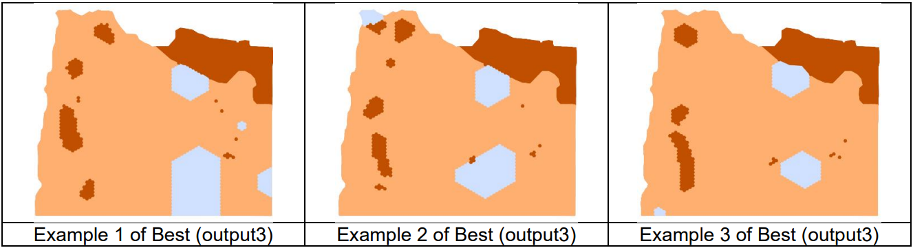Figure 3: Three different examples of the Best (output3) layer produced by CLUZ, based on ten runs, 1,000,000 iterations, a BLM value of 0.2 and Zone 1 vs Zone 2 boundary cost of 0.5.

8) There are two ways to ensure that Marxan with Zones will find efficient solutions to a particular planning problem: increase the number of runs and increase the number of iterations per run. In general, increasing the number of iterations is more effective but you can investigate the effects of using different numbers of runs and iterations with the Calibrate Marxan parameters module.

Based on previous results, we know that using 100,000,000 iterations for this analysis produces efficient results. So, from the CLUZ menu choose Launch Marxan again and change the number of iterations to 100000000 and click on Start Marxan with Zones.

These ten runs will take much longer because you have increased the number of iterations a hundred-fold. However, the results will be much more efficient. In particular, you will probably see that instead of having a patch of Zone 1 planning units next to the existing PA, there is a patch of Zone 2 planning units, i.e., the more expensive extension to the protected area that Marxan with Zones identified in Step 5 has now been replaced by a new OECM.

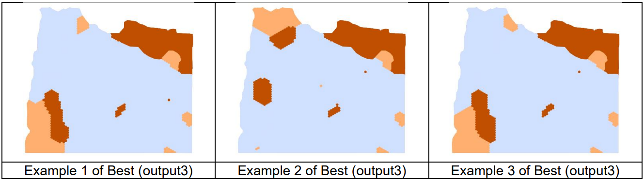Figure 4: Four different examples of the Best (output3) layer produced by CLUZ to display the results from an analysis, based on ten runs, 100,000,000 iterations, a BLM value of 0.2 and Zone 1 vs Zone 2 boundary cost of 0.5. Marxan with Zones produces different results each time it is run, so your results for Output 3 will differ from those shown above but should be similar.

You have now finished this CLUZ tutorial. You will have seen how to run Marxan with Zones through CLUZ by importing and updating CLUZ files created to run Marxan, and how to update the status and costs of each planning unit for each management zone. You will also have seen how to influence the spatial pattern of different zones by manipulating zone-specific boundary costs, and how this often requires running Marxan with Zones for longer to produce better results.