A tutorial for using CLUZ with QGIS

Exercise 1: An introduction to CLUZ

CLUZ is a plugin for QGIS that lets people design conservation landscapes and seascapes based on the principles of systematic conservation planning. It can be used for on-screen terrestrial and marine spatial planning and also acts as a link for the Marxan and Marxan with Zones spatial prioritisation software packages. CLUZ was funded by the UK Government's Darwin Initiative.

In this exercise you will first download the relevant files and save the QGIS project file that you will use in this exercise. In the second section you will view the CLUZ files and you will use these in the third section to carry out on-screen conservation planning to meet the required conservation targets. In the fourth section you will run Marxan through CLUZ to produce more efficient conservation plans.

Section 1a - Setting up Marxan, CLUZ and QGIS

1) Obtain Marxan from the University of Queensland website https://marxansolutions.org/ by downloading the Version 4.06 zip file. YOU SHOULD PLACE MARXAN IN A FOLDER WHERE YOU HAVE PERMISSION TO WRITE FILES. As part of running Marxan, CLUZ needs to update the Marxan input file and so needs access to write in the folder where Marxan is located.

2) CLUZ v3 requires version 3.0 or later of QGIS so make sure you have a suitable version installed. Open QGIS, in the Plugins menu select Manage and Install plugins... dialog box and scroll down the list of plugins until you reach CLUZ. Select CLUZ in the list and click on Install plugin. Close the dialog box. You will see the CLUZ menu and eight buttons have been added to the toolbar.

3) Obtain the CLUZ tutorial files by downloading the cluz_ex1.zip file from the link below and saving it in a suitable folder (your Internet browser may warn you about downloading zip files but these CLUZ files are safe). Unzip the tutorial files by right-clicking on the zip file and choosing Extract All...

CLUZ Exercise 1 data (cluz_ex1.zip)

Section 1b - Viewing the CLUZ files

CLUZ provides a set of tools that allow users to identify a portfolio of planning units that, when combined, meet specified conservation targets. To do this CLUZ uses three files that describe the planning units, the distributions of the conservation features and the conservation target for each conservation feature.

A fourth file describes the location of these files and sets where the Marxan input and output data are stored. In this section you will view and familiarise yourself with these four files.

1) In QGIS go to the CLUZ menu and choose View and edit CLUZ setup file. This will open the File Settings dialog Box.

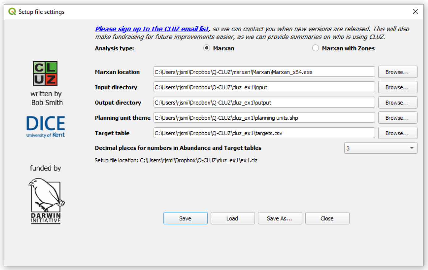
2) The File Settings dialog box will appear and you can use this to set the location of each specified file and folder. Start by clicking on the Browse button next to the Marxan location input. Navigate to the folder where you saved Marxan and choose Marxan_x64.exe.

3) Repeat the process to set the paths for the CLUZ data contained in the cluz_ex1 folder that you extracted from the zip file. Set the input directory as \cluz_ex1\input, the output directory as \cluz_ex1\output, the planning unit layer as \cluz_ex1\planning units.shp and the target table as \cluz_ex1\targets.csv. Set the Decimal places for numbers in Abundance and Target table as 3. Click on the Save As button and save the file as ex1.clz in the cluz_ex1 folder.

This will add and display the planning unit shapefile to the Table of Contents. Click the Close button.

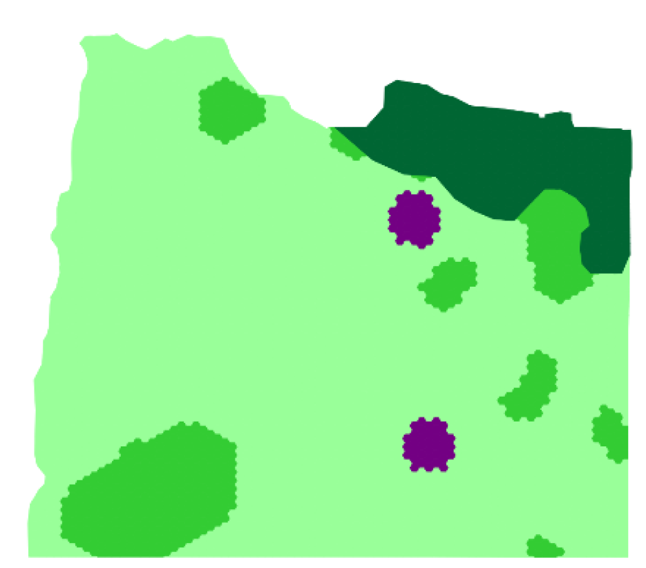
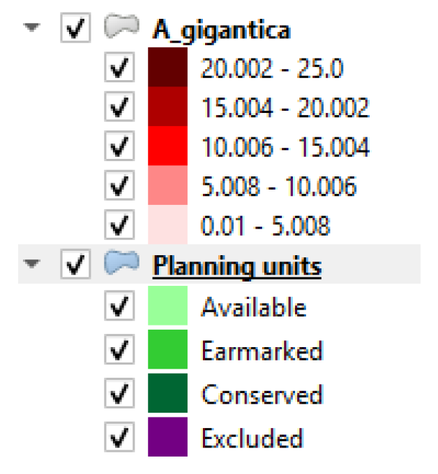
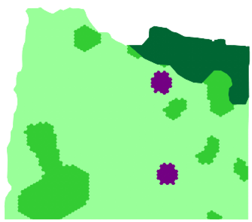
4) You will see that the theme consists of a number of hexagonal planning units (there are 4661 in all) that are coloured according to their conservation status (Available, Earmarked, Conserved and Excluded). In the northeast of the study region there is a patch of Conserved units and two smaller patches of Excluded units are located below the Conserved units.

5) Right-click on the name Planning units in the Table of Contents and select Open Attribute Table from the drop-down menu. You will see that the table contains five fields.

The Unit_ID field contains a unique numerical ID value for each planning unit, the Area field gives the area of each unit in hectares. The Cost field gives the cost of including the unit in any conservation portfolio (which in this case is set as the same as its Area, as we want Marxan to minimise the area selected) and the Status field that describes the conservation status of each unit. The Previous field is not a required field in CLUZ but you will use the information in that field for this tutorial exercise.

6) Close the Planning units attribute table and click on the Open Target Table button to display a table containing 8 fields. The Id field lists the numeric ID of each conservation feature and the Name field in the target table gives the full name of the feature. The Target field gives the required amount of each feature that should be represented in the final portfolio and the Spf field lists the species penalty factor (this will be explained in more detail later).

The Ear+Cons field lists the amount of each feature that is found in units that have Earmarked or Conserved status. The Total field lists the total amount of each feature in all of the units and the PC_target shows the percentage of the target that has been reached, based on the Ear+Cons and Target fields. The Type field is not a required CLUZ field but it can be used to distinguish between different types of conservation feature when setting the target values.

Notice the two conservation features with a type value of 0. These are landcover types with little or no conservation value and so their target values have been set as 0. This means that only 19 of the conservation features have targets set and the value of --1 will appear in the PC_target field for those features with a target value of 0.

Notice also that values in the PC_target field are colour coded. They are red if the target has not been met (value is less than 100%), green if the target has been met and grey if the target is 0.

7) Close the target table to return to the main QGIS window. The data listing how much of each conservation feature is found in each planning unit is stored in the Marxan file puvspr2.dat which is in the input folder. To view these data, click on the Open Abundance Table button and you will see a dialog box listing the names and ID values of the 21 conservation features. Select all of these features and click on the OK button to show the abundance table.

The first field is identical to the PU_ID field in the unit layer table, whereas each of the other fields contains data on the abundance of a particular conservation feature found in each planning unit. Each of the fields containing data on a particular feature has the column name "F_" followed by their id value. Close the table to return to the main QGIS window.

Section 1c - On-screen conservation planning

CLUZ is designed as an interface for Marxan but it can also be used on its own to carry out on-screen conservation planning. It lets the user change the conservation status of the different planning units and investigate how this affects the number of targets met by the portfolio of planning units. It also lets the user refine portfolios identified by Marxan to incorporate expert opinion. The main set of tools for on-screen planning is found on the Change Status panel, so this section explores these in more detail.

The status of each planning unit can either be set as Conserved, Earmarked, Available or Excluded. Conserved units are those that fall within an existing protected area (PA), or other types of conservation area, and so already form part of the conservation portfolio. Excluded units are those that are unsuitable for ecological, political or other reasons and so will not form part of any portfolio.

This means that most of the conservation planning that you will do involves changing the status of Available and Earmarked units. Available units are those that could form part of a portfolio but are not presently selected. Earmarked units are those that have been earmarked for conservation, i.e. they do not form part of an existing PA but they are part of the conservation portfolio that is being investigated.

Designing a whole conservation area network through on-screen conservation planning can be quite laborious. So, in this exercise you will first add information from a previous conservation planning exercise and then use on-screen planning to meet the only unmet target.

1) Click on the Open Target Table button to remind yourself of how well the current protected area (shown in dark green as Conserved) meets the targets. Notice that eight of the conservation features are completely unrepresented (0.000%) and another six features have not met their targets. Click on Close.

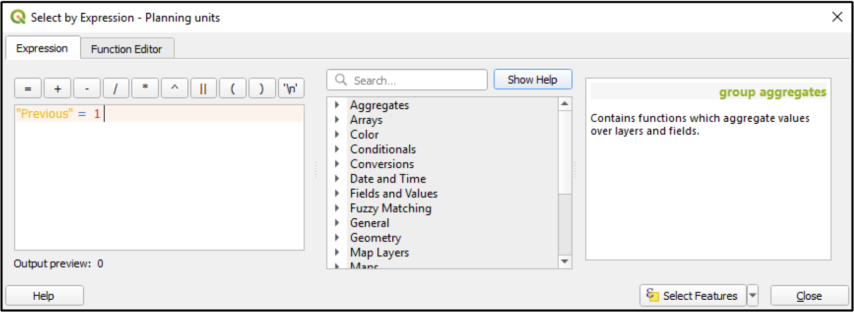
2) You will now load the results from the previous conservation planning exercise, which are stored in the Previous field (previously selected planning units are coded with a "1"). Right-click on the name Planning units in the Table of Contents and select Open Attribute Table from the drop-down menu. Now click on the Select features using an expression button . In the expression box type "Previous" = 1 and then click on the Select feature button.

Click on Close and then close the Attribute table and return to the planning units in the View.

You will see that you have selected a number of patches of planning units, highlighted in yellow. These planning units were selected in a previous conservation planning exercise and you will now set their status to Earmarked, to show that they could be future conservation areas. Do this by clicking on the Change planning unit status button .

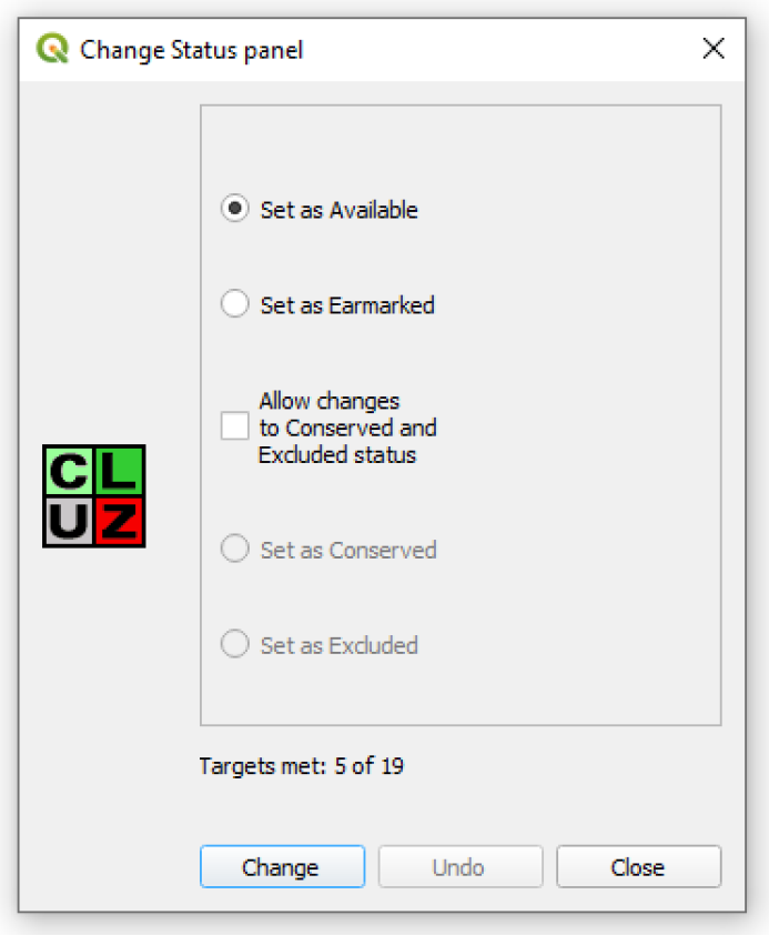
The panel shows the number of abundance targets that have been met by the present portfolio, based on the values in the Target and Ear+Cons fields in the target table. In this case, it will show that 5 of the 19 targets have been met.

3) CLUZ assumes that you will only want to set the status of Conserved and Excluded units at the beginning of the process and that these units are likely to remain unchanged during the rest of the on-screen planning process. This is why the option to set the required status as Conserved or Excluded is not automatically shown when you open the Change Status panel.

If you want to set the status of selected units to Conserved or Excluded, or if you want to change the status of Conserved or Excluded units, then you need to click on the Allow changes to Conserved and Excluded status checkbox . You will NOT need to do this for this tutorial.

4) Now click on the Change button in the Change status panel and notice how the selected Available units have been changed to Earmarked status (as shown in the picture on the right). The number of Targets met is now 18 of 19.

Close the Change Status panel and click on the Open Target Table button . By looking at the PC_target field you can identify that all but one of the targets have now been meet. The only conservation feature with an unmet target is A. gigantica, a species of plant found in the west of the planning region.

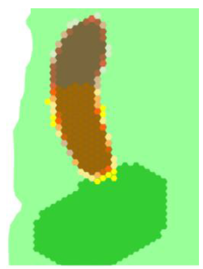
5) To identify where best to meet the target for A. gigantica, you need to look at its distribution. Go to the CLUZ menu and choose Display distribution of conservation features. Select 107 -- A_gigantica, from the list in the dialog box and click on OK. It will show that this species is found in the west of the planning region, just north of a patch of Earmarked planning units.

6) You will now use the Change Status panel to carry out on-screen conservation planning to meet the final target. Click on the Change planning unit status button and move it so it is not covering the planning unit layer. Select the Earmarked Radio button

7) Click on the Select features tool and from the drop-down menu, choose Select Features by Polygon . The target is under half of the distribution of A. gigantica (2000 ha out of a total area of 4446 ha). To meet this, it makes sense to extend the patch of Earmarked planning units that lies just south of where A. gigantica is found, creating one large conservation area.

Before you start digitising, check that the Planning units theme is active. You can tell this because the name of the active layer has a grey background in the Layers Panel on the left of the screen. If this theme is not active then click on its name in the Layer Panel. This step is important because the Select features tool only selects features in the active layer.

Now move the mouse icon to the bottom of the A. gigantica patch and left-click once to start on-screen digitising a polygon. Then move the mouse icon and keep on left-clicking to set the boundaries of a polygon so that it covers the bottom half of the distribution polygon.

Once you have finished digitising the polygon boundary, right click and the planning units you have specified will be selected (as shown in the picture on the right). These units will turn bright yellow but most of them are underneath the A. gigantica distribution layer, so you will see a more subtle colour change because this distribution layer is slightly transparent.

8) Turn off the A. gigantica distribution layer to make the planning unit layer underneath visible. Click on the Change button in the Change status panel and notice how the selected Available units now have Earmarked status (as shown in the picture on the right). Check to see whether adding the selected units has met the final target. If you have not met the target, then add a few more planning units by repeating the process in steps 6 to 7. Once, you have met the target then remove the A. gigantica distribution layer from the View.

9) Once you are happy with your final portfolio, in the QGIS Project menu select Import/Export, then Export Map to Image... and click on Save to save the results as a file named onscreen.png in the cluz_ex1 folder.

Section 1d - Using Marxan to select conservation portfolios

In the previous section you will have seen that it is possible to use on-screen techniques to design a conservation portfolio. However, the results of these exercises tend to be inefficient and are more difficult to produce when dealing with a large number of targets. In this section you will use Marxan to produce a quicker and more efficient solution.

1) To convert the portfolio back to the original version, click on the Change Earmarked units to Available button . This will show only the patch of Conserved units and the two patches of Excluded units. Remove any other layers so that only the planning unit layer is present.

2) Marxan only uses specifically formatted text files to input the data it needs, so the first step is to convert the CLUZ data into Marxan format. Go to the CLUZ menu, choose the Create Marxan input files option and click on all the checkboxes, so that you will produce all three of the additional files used by Marxan.

Selecting the Boundary file (bound.dat) checkbox gives you the option to select the Include planning region boundaries option. DO NOT click this Include planning region boundaries checkbox, so that the edges of units that are not shared (i.e., form the boundary of the study region) are not included in the boundary.dat file. Including the external edges makes it less likely Marxan will select planning units at the edge of the planning region.

Click on OK to produce all three of the additional files needed by Marxan. These will be stored in the input folder you specified in the setup file, together with the puvspr2.dat file that was already stored in the input folder.

You are now ready to run Marxan. Remember that Marxan will only use data from the text files you have just created. If you change any of the CLUZ data you must update these text files by repeating the process above before running Marxan.

3) In the CLUZ menu choose Launch Marxan. Under Standard options in the dialog box, you will see that the number of iterations has been set as 1000000 and the number of runs as 10. Increasing the number of iterations and runs will generally improve the efficiency of the portfolios that Marxan identifies but also increases processing time.

In this tutorial you will use these default values to reduce the time Marxan spends processing the data. Set output1 as the Output file name and leave the Include boundary cost (BLM) and Produce extra Marxan outputs checkboxes unchecked . The Produce extra Marxan outputs option saves files describing the results from each run, which are not needed for this exercise.

Click on Start Marxan and the Marxan dialog box should appear. The Marxan dialog box will show that the data are being inputted and will then give details on each of the 10 runs.

NB If you are a running CLUZ on a computer with high security settings, your system might not let CLUZ run Marxan. If that happens Marxan will produce the error message "Input file input.dat not found. Aborting program" and/or it will look as though it has frozen. To overcome this problem, you can run Marxan yourself by using Windows Explorer to locate Marxan (the file path is specified in your CLUZ setup file) and double clicking on it. Marxan should now run and, once it is finished, CLUZ will display the results.

4) Return to QGIS and two new layers should be displayed. The Best (output1) layer shows a portfolio of units in magenta. This portfolio was the most efficient of the 10 solutions produced by Marxan. Make the Best layer (output1) invisible and then inspect the SF_Score (output1) layer.

The summed layer shows the number of times that each unit was selected to be part of one of the 10 portfolios. This is similar to an irreplaceability score, with the most important units being included in the largest number of portfolios.

Click on the Open Marxan results table button to view the text file that Marxan has saved in the \output folder. This lists each feature, its target and whether the target was met. In particular, Target met states yes or no and MPM shows the Minimum Proportion Met of the target, i.e. if the MPM is less than 0 then the target has not been met.

5) Make the Best layer active and open the Attribute Table . Note that two fields have been added to the table. The Best field contains the word Selected for the units that were included in the most efficient portfolio and SF_Score gives the irreplaceability score for each unit. The information in these fields will be overwritten every time you run Marxan.

6) You have now completed Analysis 1. In the next sections you will learn how to save and calculate different characteristics of this Analysis and three others, so you can investigate the results of changing different parameters.

As a first step, remove the SF_Score and Best layer from the QGIS window and then click on the Change the status of the Best units to Earmarked button. This updates the portfolio so that it includes the planning units identified by Marxan in the last analysis. In the QGIS Project menu select Import/Export and Export Map to Image.... Then click on Save to save the screen view as a file named area_0.png in the cluz_ex1 folder.

7) You will now produce statistics describing this portfolio of Earmarked and Conserved planning units by going to the CLUZ menu and selecting Calculate portfolio characteristics. Make sure the tick boxes are selected for the options to calculate the Planning unit details and Spatial details (patch sizes and boundary length). Also click on the Selection frequency details of Available and Earmarked planning units option, make sure the Field contains values for SF_Score and set the Number of runs used in analysis as 10, because you used 10 runs in the Marxan analysis and so the maximum selection frequency value cannot be higher than 10.

You will now see displayed three separate tables (on three different tabs) giving details on the portfolio. Write in the values in the Results table on page 7 for Analysis 1. Note that the Total cost and area values are the same because this analysis used planning unit area as the planning unit cost metric (so that Marxan minimises the area selected when meeting targets).

8) You have now finished Analysis 1 and so need to return the portfolio to its original state. To convert the portfolio back to the original version, click on the Change Earmarked units to Available button . This will show only the patch of Conserved units and the two patches of Excluded units. Remove any other layers so that only the planning unit layer is present.

9) The portfolio identified by Marxan may be efficient but it is very fragmented and would be ecologically unviable and expensive to manage. Marxan can overcome this problem by including a boundary cost that favours the identification of portfolios that form patches of planning units. Do this by choosing Launch Marxan from the CLUZ menu again but this time, click the Include boundary cost (BLM) on and set a value of 0.25. This is Analysis 2.

10) Repeat steps 6 to 9 to fill in the table below for Analysis 2 and use Import/Export and Export Map to Image... save the best output. Name the file area_0_25.png.

Now go through the same process for two more analyses that use higher BLM values, so that Analysis 3 uses a BLM value of 0.5, and Analysis 4 uses a BLM value of 2. Table 1 below gives the names you should use for the screenshot image files.

11) Compare the four best portfolios you have produced in terms of efficiency (number of planning units selected) and fragmentation (number of patches). You should see that as you increase the BLM value, the portfolio cost and area increase and the results consist of fewer, larger patches. This is because selecting large patches that best the meet the targets is less efficient than choosing the individual planning units that best the meet the targets.

You should also see from the selection frequency scores, that more planning units are never selected or always selected. This is because when you add an extra constraint to your analysis (the requirement to identify larger patches), there are fewer ways to achieve good results. This means the results of each run are more similar, so the same planning units tend to get selected